Introduction

Artificial neural networks are a machine learning discipline roughly inspired by how neurons in a human brain work. In the past decade, there has been a huge resurgence of neural networks thanks to the vast availability of data and enormous increases in computing capacity (Successfully training complex neural networks in some domains requires lots of data and compute capacity). There are various types of neural networks (Feedforward, recurrent, etc.). In this tutorial, we discuss feedforward neural networks (FNN), which have been successfully applied to pattern classification, clustering, regression, association, optimization, control, and forecasting (Jain et al. 1996). We will discuss biological neurons that inspired artificial neural networks, review activation functions, classification/regression problems solved by neural networks, and the backpropagation learning algorithm. Finally, we construct a FNN to solve a regression problem using car purchase price prediction dataset.

Agenda

In this tutorial, we will cover:

1. Introduction
2. Inspiration for artificial neural networks
3. Perceptron
4. Activation functions
5. Supervised learning
6. Loss/Cost function
7. Backpropagation Learning algorithm
8. Get Data
9. Solve a simple regression problem using car purchase price prediction dataset via FNN in Galaxy
10. Conclusion

Inspiration for artificial neural networks

A neuron is a special biological cell with information processing ability (Jain et al. 1996). Figure 1 shows a biological neuron. It has a cell body and two outreaching tree-like branches: axon and dendrites. A neuron receives signals from other neurons through its dendrites, and transmits signals generated by its cell body to other neurons via its axon. A synapse is a place of contact between two neurons, an axon strand of one neuron and a dendrite strand of another neuron. A synapse can either enhance or inhibit the signal that passes through it. Learning occurs by changing the effectiveness of synapse. If the signals received exceeds a threshold, the neuron fires, i.e., it transmits a signal to other neurons. If not, it will not fire.

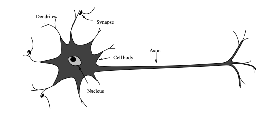
Cerebral cortex, the outer most layer of the brain, is a sheet of neurons about 2 to 3 mm thick, with a surface area of about 2,200 \(cm^{2}\). Cerebral cortex has about \(10^{11}\) neurons. Each neuron is connected to \(10^{3} to 10^{4}\) neurons. Hence, a human brain has around \(10^{14} to 10^{15}\) connections. Neurons communicate by a short train of signals, usually milliseconds in duration. The frequency in which the signals are transmitted can be up to several hundred Hertz, which is millions of times slower than an electronic circuit. However, complex tasks, such as face recognition are made within a few hundred milliseconds. This implies that computation involved cannot take more than 100 serial steps, i.e., brain runs parallel programs that are about 100 steps long for such complex perceptual tasks. The amount of information sent from one neuron to another is also very small. This implies that critical information is not transmitted directly, but is captured by the interconnections. What enables slow computing elements in the brain to perform complex tasks so quickly is the distributed computation and representation nature of the brain (Jain et al. 1996).

Perceptron

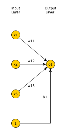
Perceptron (Rosenblatt 1957) is the oldest neural network still in use today. It’s a form of a feedforward neural network, in which the connections between the nodes do not form a loop. It accepts multiple inputs, each input is multiplied by a weight, and the products are added up. The weights simulate the role of synapse in biological neurons (to enhance or inhibit a signal). A bias value is then added to the result before it is passed to an activation function. An activation function simulates the neuron firing or not. For example, in a binary step activation function, if the sum of weighted inputs and bias is greater than zero, the neuron output is 1 (it fires). Else, the neuron output is 0 (it does not fire). Bias allows us to shift the activation function.

\[f(x) = \left\{ \begin{array}{ll} 1 & \mbox{if } \boldsymbol{x} \cdot \boldsymbol{w} + b \geq 0 \\ 0 & \mbox{otherwise } \end{array} \right.\]

Figure 2 shows a Perceptron, a single layer FNN, where the input is 3 dimensional (input layer has 3 nodes), and output is 1 dimensional (output layer has 1 node).

In supervised learning, we are given a set of input-output pairs, called the training set. Given the training set, the learning algorithm (iteratively) adjusts the model parameters (weights and biases), so that the model can accurately map inputs to outputs. The learning algorithm for Perceptron is very simple and reduces the weights (via a small learning rate multiplier) if the predicted output is more than the expected output and increases them otherwise (Rosenblatt 1957).

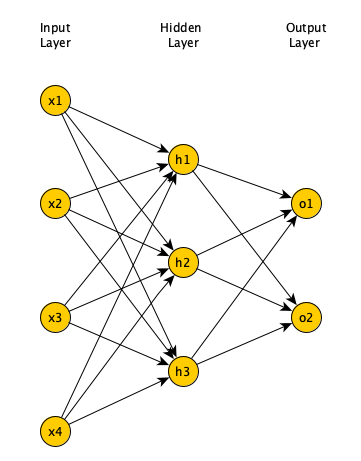
Minsky and Papert showed that a single layer FNN cannot solve problems in which the data is not linearly separable, such as the XOR problem (Newell 1969). Adding one (or more) hidden layers to FNN enables it to solve problems in which data is non-linearly separable. Per Universal Approximation Theorem, a FNN with one hidden layer can represent any function (Cybenko 1989), although in practice training such a model is very difficult (if not impossible), hence, we usually add multiple hidden layers to solve complex problems.

The problem with multi-layer FNN was lack of a learning algorithm, as the Perceptron’s learning algorithm could not be extended to multi-layer FNN. This along with Minsky and Papert highlighting the limitations of Perceptron resulted in sudden drop in interest in neural networks (referred to as AI winter). In the 80’s the backpropagation algorithm was proposed (Rumelhart et al. 1986), which enabled learning in multi-layer FNN and resulted in a renewed interest in the field.

In a multi-layer neural network, we have an input layer, an output layer, and one or more hidden layers (between input and output layers). The input layer has as many neurons as the dimension of the input data. The number of neurons in the output layer depends on the type of the problem the neural network is trying to solve (See Supervised learning section below). The more hidden layers that we have (and the more neurons we have in each hidden layer), our neural network can estimate more complex functions. However, this comes at the cost of increased training time (due to increased number of parameters) and increased likelihood of overfitting. Overfitting happens when a model captures the details of the training data, performs well on the training data, but is unable to perform well on data not used in the training. The neural network, hence, cannot generalize to unseen data. There are regularization techniques that can prevent that (Kukacka et al. 2017) but they are outside the scope of this tutorial.

Activation functions

There are many activation functions besides the step function used in Perceptron (Nwankpa et al. 2018). Figure 4 shows some of the more common activation functions.

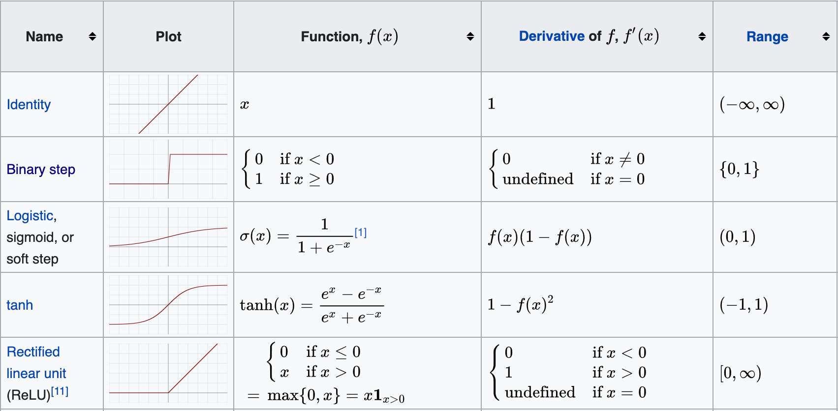
Linear activation function is used in the output layer of a network when we have a regression problem. It does not make sense to use it in all layers, as such multi-layer network can be reduced to a single layer network. Also, networks with linear activation functions cannot model non-linear relationships between input and output.

Binary step activation function is used in Perceptron. It cannot be used in multi-layers networks as they use back propagation learning algorithm, which changes network weights/biases based on the derivative of the activation function, which is zero. Hence, there would no weights/biases updates in back propagation.

Sigmoid activation function can be used both at the output layer and hidden layers of a multilayer network. They allow the network to model non-linear relationships between input and output. The problem with Sigmoid activation function is that the derivative values away from the origin are very small and quickly approach zero. In a multi layer network, in order to calculate weight updates in layers closer to the input layer, we use the chain rule which requires multiplying multiple Sigmoid derivative values (formula given in Backpropagation learning algorithm section below). Multiplying multiple small numbers results in a very small number, meaning that the weight updates will be minimal and the learning algorithm will be very slow. This is known as the vanishing gradient problem. In networks with many hidden layers (so called deep networks), we generally avoid Sigmoid and use ReLU activation function.

Hyperbolic tangent (or tanh), similar to Sigmoid function, is a soft step function. But its range is between -1 and 1 (instead of 0 and 1). One benefit of tanh over Sigmoid is that its derivative values are larger, so it suffers less from the vanishing gradient problem.

Finally, ReLU (Rectified Linear Unit) is an activation function popular is deep neural networks. Since it does not suffer from vanishing gradient problem, it is preferred to Sigmoid or tanh. Sigmoid or tanh can still be used in the output layer of deep networks.

Supervised learning

In supervised learning a training set is defined as \({(\boldsymbol{x^{(1)}}, \boldsymbol{y^{(1)}}), ((\boldsymbol{x^{(2)}}, \boldsymbol{y^{(2)}}), ..., ((\boldsymbol{x^{(m)}}, \boldsymbol{y^{(m)}})}\) and each pair \((\boldsymbol{x^{(i)}}, \boldsymbol{y^{(i)}})\) is called a training example. m is the number of training examples and \(\boldsymbol{x^{(i)}}\) is called feature vector or input vector. Each element of the vector is called a feature. Each \(\boldsymbol{x^{(i)}}\) corresponds to a label \(\boldsymbol{y^{(i)}}\). We assume there is an unknown function \(\boldsymbol{y} = f(\boldsymbol{x})\) that maps the feature vectors to labels. The goal of supervised learning is to use the training set to learn or estimate f. We call this estimated function \(\hat{f}(\boldsymbol{x})\). We want \(\hat{f}(\boldsymbol{x})\) to be close to \(f(\boldsymbol{x})\) not only for training set, but for training examples not in training set (Bagheri 2020).

When the label is a numerical variable, we call the problem a regression problem, and when it’s a categorical variable, we call it a classification problem. In classification problems, the label can be represented by the set \(\boldsymbol{y^{i}} \in {1,2,...,c}\), where each number is a class label and c is the number of classes. If c=2, the class labels are mutually exclusive, we call it a binary classification problem. If c > 2, and the labels are mutually exclusive, we call multiclass classification problem. If labels are not mutually exclusive, we call it a multilabel classification problem (Bagheri 2020).

We use a method called one-hot encoding to convert binary and multiclass classification class label numbers into binary values. We convert the scalar label y into a vector \(\boldsymbol{y}\) which has c elements. When y is equal to k, the k-th element of \(\boldsymbol{y}\) is one and all other elements are zero. When labels are not mutually exclusive, we use another method called multi-hot encoding. Suppose we are doing a multilabel image classification, where an image can have a dog, panda, or cat in it. We represent the label by a vector of 3, and if dog and cat are present in the image, first and third element of the vector are one and the second element is zero (Bagheri 2020).

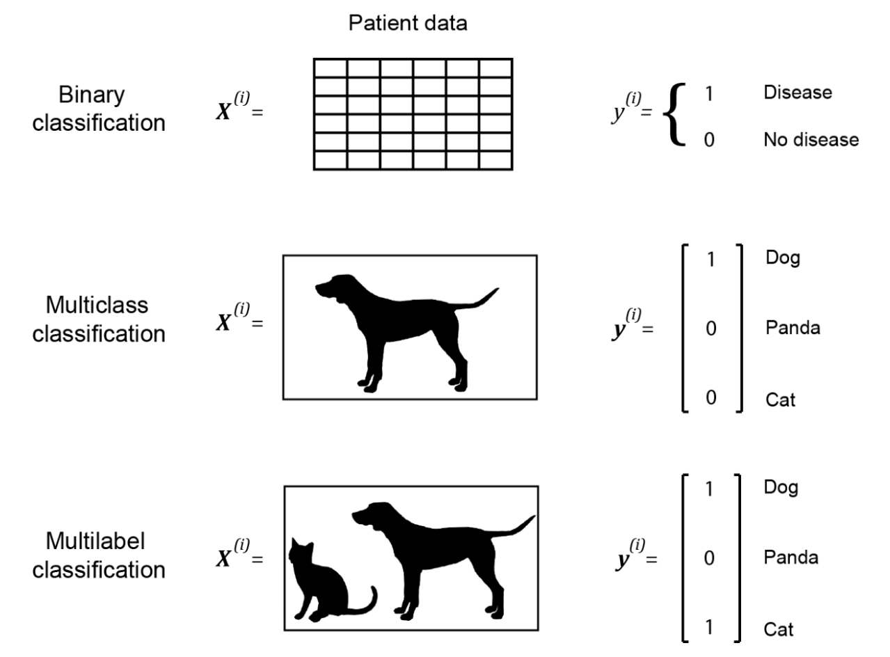
Figure 5 shows examples of binary, multiclass, and multilabel classification problems and their associated one-hot encoded or multi-hot encoded labels. The output layer of a neural network for binary classification usually has a single neuron with Sigmoid activation function. If the neuron’s output is greater than 0.5, we assume the output is 1, and otherwise, we assume the output is 0. For multilabel classification problems, the output layer of the neural network usually has as many neurons as the number of classes and the neurons use Sigmoid activation function. Again, we use a threshold of 0.5 to determine whether the output of each neuron is 1 or 0. For multiclass classification problems, the output layer usually has as many neurons as the number of classes. However, instead of Sigmoid, we use a Softmax activation function, which takes the input to all the neurons in the output layer, and creates a probability distribution, so, the sum of outputs of all output layer neurons adds up to 1. The neuron with the highest probability denotes the predicted label.

Loss/Cost function

During training, for each training example in the training set \((\boldsymbol{x^{(i)}}, \boldsymbol{y^{(i)}})\), we present the feature vector \(\boldsymbol{x^{(i)}}\) to the neural network, and compare the network’s predicted output \(\boldsymbol{\hat{y}}\) with the corresponding label \(\boldsymbol{y^{(1)}}\). We need to define a loss function to objectively measure how much the network’s predicted output is different than the expected output (the corresponding label). We use the cross entropy loss function for classification problems, and quadratic loss function for regression problems.

For multiclass classification problems, the cross entropy is calculated as below

\[\mathcal{L}(\boldsymbol{\hat{y}^{(j)}}, \boldsymbol{y^{(j)}}) = - \sum_{i=1}^{c} \boldsymbol{y_{i}^{(j)}}ln(\boldsymbol{\hat{y}_{i}^{(j)}})\]

You can find the cross entropy formula for binary and multilabel classifications in Bagheri 2020. They are just special cases of multiclass cross entropy and are not give here for the sake of brevity.

The loss function is calculated for each training example in the training set. The average of the calculated loss functions for all training examples in the training set is the cost function. For multiclass classification problems, the cost function is calculated as below (again refer to Bagheri 2020 for binary classification and multilabel classification formulas).

\[J(\boldsymbol{W}, \boldsymbol{b}) = - \frac{1}{m} \sum_{j=1}^{m} \sum_{i=1}^{c} \boldsymbol{y_{i}^{(j)}}ln(\boldsymbol{\hat{y}_{i}^{(j)}})\]

For regression problems, the quadratic loss function is calculated as below:

\[\mathcal{L}(\boldsymbol{\hat{y}^{(j)}}, \boldsymbol{y^{(j)}}) = \frac{1}{2} \| \boldsymbol{y^{(j)}} - \boldsymbol{\hat{y}^{(j)}} \| ^ 2\]

Similarly, the quadratic cost function (or Mean Squared Error (MSE)) is the average of the calculated loss functions for all training examples in the training set.

\[J(\boldsymbol{W}, \boldsymbol{b}) = \frac{1}{2m} \sum_{j=1}^{m} \| \boldsymbol{y^{(j)}} - \boldsymbol{\hat{y}^{(j)}} \| ^ 2\]

Backpropagation Learning algorithm

The backpropagation algorithm Rumelhart et al. 1986 is a gradient descent technique. Gradient descent aims to find a local minimum of a function by iteratively moving in the opposite direction of the gradient (i.e., the slope) of the function at the current point. The goal of a learning in neural networks is to minimize the cost function given the training set. The cost function is a function of network weights and biases of all the neurons in all the layers. Backpropagation iteratively computes the gradient of cost function relative to each weight and bias, then updates the weights and biases in the opposite direction of the gradient, to find a local minimum.

In order to specify the formula for backpropagation, we need to define the error of the \(i^{th}\) neuron in \(l^{th}\) layer of a network for the \(j^{th}\) training example as follows (where \(z_{i}^{[l](j)}\) is the weighted some of input to the neuron, and \(\mathcal{L}\) is the loss function):

\[\delta_{i}^{[l](j)} = \frac{\partial \mathcal{L}(\boldsymbol{\hat{y}^{(j)}}, \boldsymbol{y^{(j)}})}{\partial z_{i}^{[l](j)}}\]

Backpropagation formulas are expressed in terms of the error defined above. Full derivation of the formulas below is outside the scope of this tutorial (Repeated use of chain rule is needed. Please refer to the excellent article by Bagheri 2020 for details). Note that in formulas below L denotes the output layer, g the activation function, \(\nabla\) the gradient, \(W^{[l]^{T}}\) layer l weights transposed, \(b_{i}^{l}\) bias of neuron i at layer l, \(w_{ik}^{l}\) weight to neuron i at layer l from neuron k from layer l-1, and \(a_{k}^{[l-1](j)}\) activation of neuron k at layer l-1 for training example j.

\[\boldsymbol{\delta}^{[L](j)} = \nabla_{\boldsymbol{\hat{y}^{(j)}}}\mathcal{L} \odot (g^{[L]})^{'} (\boldsymbol{z}^{[L](j)}) = \boldsymbol{\hat{y}^{(j)}} - \boldsymbol{y^{(j)}}\] \[\boldsymbol{\delta}^{[l](j)} = W^{[l+1]^{T}} \boldsymbol{\delta}^{[l+1](j)} \odot (g^{[l]})^{'} (\boldsymbol{z}^{[l](j)})\] \[\frac{\partial L}{\partial b_{i}^{[l]}} = \boldsymbol{\delta}_{i}^{[l](j)}\] \[\frac{\partial L}{\partial w_{ik}^{[l]}} = \boldsymbol{\delta}_{i}^{[l](j)} a_{k}^{[l-1](j)}\]

As you can see, we can calculate the error at the output layer for sample j using the first equation. Afterwards, we can calculate the error in the layer right before the output layer for sample j using the second equation. The second equation is recursive, meaning that we can calculate the error in any layer, given the error values for the next layer. This backward calculation of the errors is the reason this algorithm is called backpropagation.

After the error values for all the layers are calculated for sample j, we use the third and fourth equations to calculate the gradient of loss function relative to biases and weights for sample j. We can repeat these steps for all the samples, average the gradients of the loss function relative to biases and weights and use the average value to update the biases and weights. This is called batch gradient descent. If we have too many samples, such calculations will take a long time. An alternative is to update the biases/weights based on the gradient of each sample. This is called stochastic gradient descent. While this is much faster than batch gradient descent, the gradient calculated based on a single sample is not a good estimate of the gradient calculated in the batch version of the algorithm. A middle ground solution is to calculate the gradient of a batch, and update the biases and weights based on the average of the gradients in the batch. This is called mini-batch gradient descent and is preferred to the other two variations of the algorithm.

Also, note that in the second equation which is recursive, we have a term that is the derivative of the activation function for that layer. The recursive nature of this equation means, calculating the error values in the layer prior to the output layer requires 1 multiplication by the derivative value; calculating the error values in two (or more) layers before the output layer requires 2 (or more) multiplication by the derivative values. If these derivative values are small, as could be the case for the Sigmoid function, the product of multiple small values will result in a very small value (e.g., 0.001). Since these error values decide the updates for biases and weights, this means the update to biases and weights in layers closer to the input layer will be very small, slowing the learning algorithm to a halt. This phenomenon is known as the vanishing gradient problem and is the reason Sigmoid function cannot be used in very deep networks (And why ReLU is so popular in deep networks).

Get Data

Hands-on: Data upload

1. Create a new history for this tutorial

   Tip: Creating a new history

   Click the new-history icon at the top of the history panel.

   If the new-history is missing:

   1. Click on the galaxy-gear icon (History options) on the top of the history panel
   2. Select the option Create New from the menu

2. Import the files from Zenodo or from the shared data library

   https://zenodo.org/record/4660497/files/X_test.tsv
   https://zenodo.org/record/4660497/files/X_train.tsv
   https://zenodo.org/record/4660497/files/y_test.tsv
   https://zenodo.org/record/4660497/files/y_train.tsv
   

   Tip: Importing via links

   • Copy the link location

   • Open the Galaxy Upload Manager (galaxy-upload on the top-right of the tool panel)

   • Select Paste/Fetch Data

   • Paste the link into the text field

   • Press Start

   • Close the window

   Tip: Importing data from a data library

   As an alternative to uploading the data from a URL or your computer, the files may also have been made available from a shared data library:

   • Go into Shared data (top panel) then Data libraries
   • Navigate to the correct folder as indicated by your instructor
   • Select the desired files
   • Click on the To History button near the top and select as Datasets from the dropdown menu
   • In the pop-up window, select the history you want to import the files to (or create a new one)
   • Click on Import

3. Rename the datasets as X_test, X_train, y_test, and y_train respectively.

   Tip: Renaming a dataset

   • Click on the galaxy-pencil pencil icon for the dataset to edit its attributes
   • In the central panel, change the Name field
   • Click the Save button

4. Check that the datatype of all the four datasets is tabular. If not, change the dataset’s datatype to tabular.

   Tip: Changing the datatype

   • Click on the galaxy-pencil pencil icon for the dataset to edit its attributes
   • In the central panel, click on the galaxy-chart-select-data Datatypes tab on the top
   • Select tabular
     • tip: you can start typing the datatype into the field to filter the dropdown menu
   • Click the Save button

Solve a simple regression problem using car purchase price prediction dataset via FNN in Galaxy

In this section, we define a FNN (Python and tutorials 2018) and train it using car purchase price prediction dataset (Grogan 2020). Given 5 attributes about an individual (age, gender, average miles driven per day, personal debt, and monthly income), and the money they spent on purchasing a car, the goal is to learn a model such that given an individual’s attributes, we can accurately predict how much money they are will spend purchasing a car. We then evaluate the trained FNN on the test dataset and plot various graphs to assess the model’s performance. Our training dataset has 723 training examples, and our test dataset has 242 test examples. Input features have been scaled to be in 0 to 1 range.

Create a deep learning model architecture

Hands-on: Model config

• Create a deep learning model architecture Tool: toolshed.g2.bx.psu.edu/repos/bgruening/keras_model_config/keras_model_config/0.4.2
  • “Select keras model type”: sequential
  • “input_shape”: (5,)
  • In “LAYER”:
    • param-repeat “1: LAYER”:
      • “Choose the type of layer”: Core -- Dense
        • “units””: 12
        • “Activation function”: relu
    • param-repeat “2: LAYER”:
      • “Choose the type of layer”: Core -- Dense
        • “units””: 8
        • “Activation function”: relu
    • param-repeat “3: LAYER”:
      • “Choose the type of layer”: Core -- Dense
        • “units””: 1
        • “Activation function”: linear
  • Click “Execute”

Input has 5 attributes: age, gender, average miles driven per day, personal debt, and monthly income. Our neural network has 3 layers. All three layers are fully connected. The last layer has a single neuron with a linear activation function, used in regression problems. Prior layers use ReLU activation function. The model config can be downloaded as a JSON file.

Create a deep learning model

Hands-on: Model builder (Optimizer, loss function, and fit parameters)

• Create deep learning model Tool: toolshed.g2.bx.psu.edu/repos/bgruening/keras_model_builder/keras_model_builder/0.4.2
  • “Choose a building mode”: Build a training model
  • “Select the dataset containing model configuration”: Select the Keras Model Config from the previous step.
  • “Do classification or regression?”: KerasGRegressor
  • In “Compile Parameters”:
    • “Select a loss function”: mse / MSE / mean_squared_error
    • “Select an optimizer”: Adam - Adam optimizer
    • “Select metrics”: mse / MSE / mean_squared_error
  • In “Fit Parameters”:
    • “epochs”: 150
    • “batch_size”: 50
  • Click “Execute”

A loss function measures how different the predicted output is from the expected output. For regression problems, we use Mean Squared Error (MSE) loss function, which averages the square of the difference between predicted and actual values for the batch. Epochs is the number of times the whole training data is used to train the model. If we update network weights/biases after all the training data is fed to the network, the training will be slow (as we have 723 training examples in our dataset). To speed up the training, we present only a subset of the training examples to the network, after which we update the weights/biases. batch_size decides the size of this subset (which we set to 50). The model builder can be downloaded as a zip file.

Deep learning training and evaluation

Hands-on: Training the model

• Deep learning training and evaluation Tool: toolshed.g2.bx.psu.edu/repos/bgruening/keras_train_and_eval/keras_train_and_eval/1.0.8.2
  • “Select a scheme”: Train and Validate
  • “Choose the dataset containing pipeline/estimator object”: Select the Keras Model Builder from the previous step.
  • “Select input type:”: tabular data
    • “Training samples dataset”: Select X_train dataset
    • “Choose how to select data by column:”: All columns
    • “Does the dataset contain header:”: Yes
    • “Dataset containing class labels or target values”: Select y_train dataset
    • “Choose how to select data by column:”: All columns
    • “Does the dataset contain header:”: Yes
  • Click “Execute”

The training step generates 3 datasets. 1) accuracy of the trained model, 2) the trained model, downloadable as a zip file, and 3) the trained model weights, downloadable as an hdf5 file. These files are needed for prediction in the next step.

Model Prediction

Hands-on: Testing the model

• Model Prediction Tool: toolshed.g2.bx.psu.edu/repos/bgruening/model_prediction/model_prediction/1.0.8.2
  • “Choose the dataset containing pipeline/estimator object” : Select the trained model from the previous step.
  • “Choose the dataset containing weights for the estimator above” : Select the trained model weights from the previous step.
  • “Select invocation method”: predict
  • “Select input data type for prediction”: tabular data
  • “Training samples dataset”: Select X_test dataset
  • “Choose how to select data by column:”: All columns
  • “Does the dataset contain header:”: Yes
  • Click “Execute”

The prediction step generates 1 dataset. It’s a file that has the predicted car purchase price for every row in the test dataset.

Plot actual vs predicted curves and residual plots

Hands-on: Check and visualize the predictions

• Plot actual vs predicted curves and residual plots Tool: toolshed.g2.bx.psu.edu/repos/bgruening/plotly_regression_performance_plots/plotly_regression_performance_plots/0.1
  • “Select input data file”: y_test
  • “Select predicted data file””: Select Model Prediction from the previous step
  • Click “Execute”

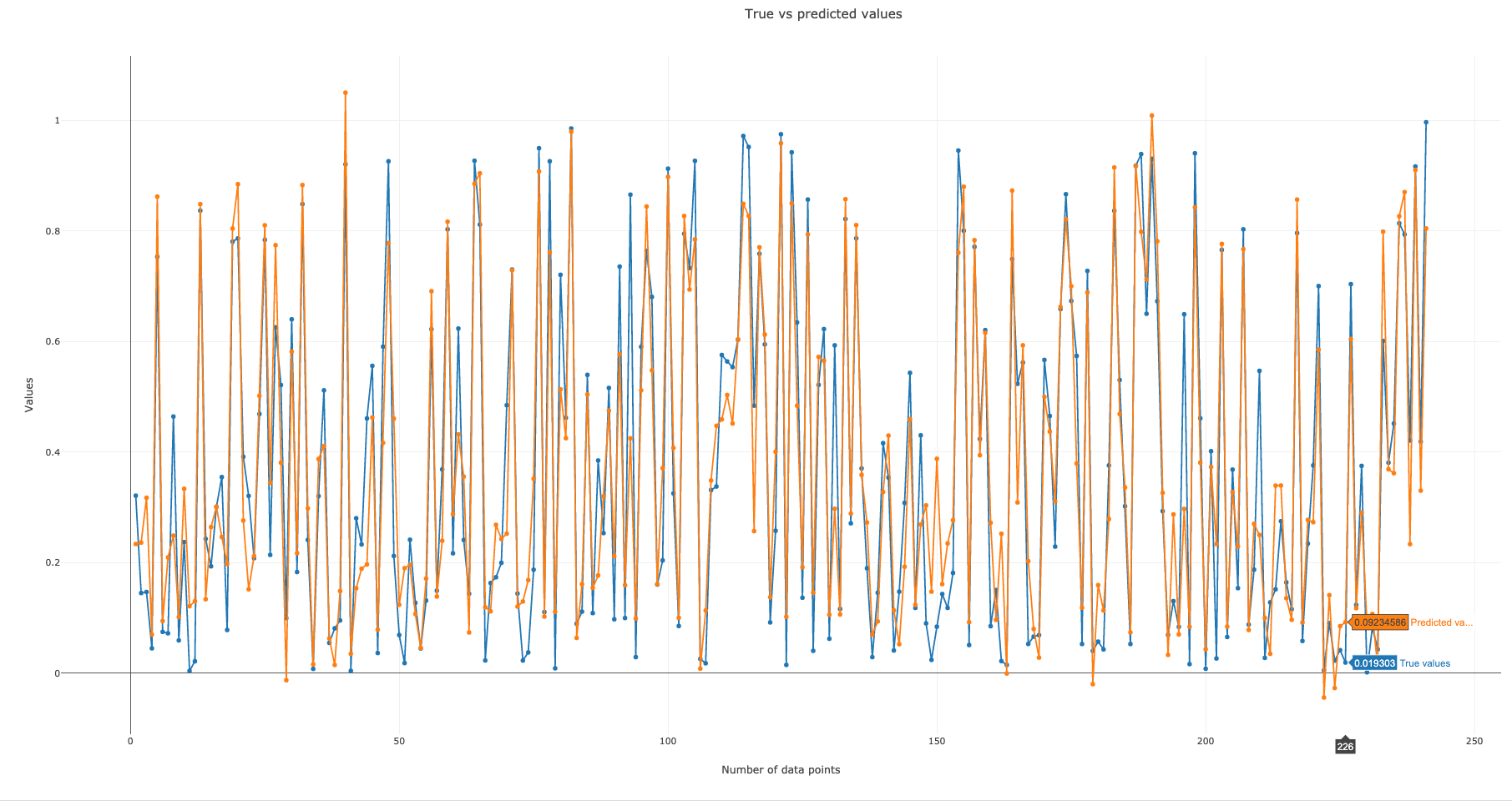
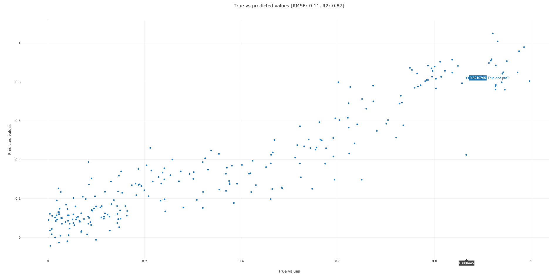
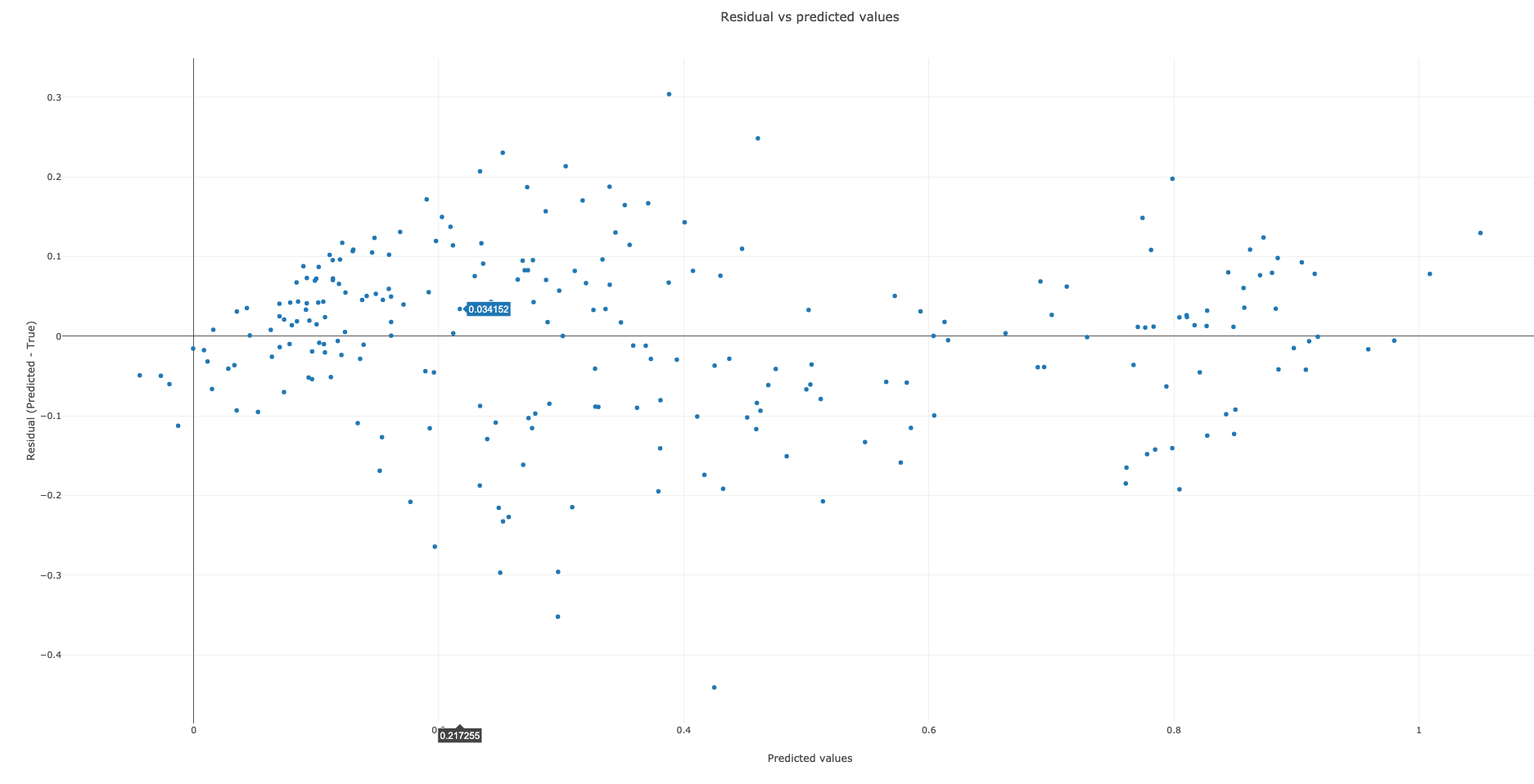
This step generates 3 graphs. The first graph (Figure 6) plots true vs predicted values. The closer the points are to each other, the better our model’s performance at predicting. The second graph (Figure 7) is a scatter plot of true vs predicted values. If our model predicts all values correctly, we would get a diagonal line (going from bottom left to upper right). The more the predicted vs true points are off this diagonal line, the worse our model’s performance at predicting. The R2 (coefficient of determination) score for our model is 0.87 (out of the best possible score of 1.0). The RMSE (root mean squared error) is 0.11. The best value for RMSE is obviously 0 for perfect prediction. The third graph (Figure 8) plots residual (predicted - true) vs predicted values. The better our model’s predictions, the closer the points to y=0 line.

Conclusion

In this tutorial, we discussed the inspiration behind the neural networks, and explained Perceptron, one of the earliest neural networks still in use today. We then discussed different activation functions, what supervised learning is, what are loss/cost functions, and how backpropagation minimizes the cost function. Finally, we implemented a FNN in Galaxy to solve a regression problem on car purchase price prediction data.

Frequently Asked Questions

Have questions about this tutorial? Check out the tutorial FAQ page or the FAQ page for the Statistics and machine learning topic to see if your question is listed there. If not, please ask your question on the GTN Gitter Channel or the Galaxy Help Forum

References

1. Rosenblatt, F., 1957 The Perceptron, a Perceiving and Recognizing Automaton Project Para. Cornell Aeronautical Laboratory. https://books.google.com/books?id=P_XGPgAACAAJ
2. Newell, A., 1969 Perceptrons. An Introduction to Computational Geometry. Marvin Minsky and Seymour Papert. M.I.T. Press, Cambridge, Mass., 1969. vi + 258 pp., illus. Cloth, 12; paper, 4.95. Science 165: 780–782. 10.1126/science.165.3895.780 https://science.sciencemag.org/content/165/3895/780
3. Rumelhart, D. E., G. E. Hinton, and R. J. Williams, 1986 Learning representations by back-propagating errors. Nature 323: 533–536. 10.1038/323533a0
4. Cybenko, G., 1989 Approximation by superpositions of a sigmoidal function. Mathematics of Control, Signals and Systems 2: 303–314. 10.1007/BF02551274
5. Jain, A. K., J. Mao, and K. M. Mohiuddin, 1996 Artificial neural networks: a tutorial. Computer 29: 31–44. 10.1109/2.485891
6. Kukacka, J., V. Golkov, and D. Cremers, 2017 Regularization for Deep Learning: A Taxonomy. CoRR abs/1710.10686: 1710.10686 http://arxiv.org/abs/1710.10686
7. Nwankpa, C., W. Ijomah, A. Gachagan, and S. Marshall, 2018 Activation Functions: Comparison of trends in Practice and Research for Deep Learning. CoRR abs/1811.03378: http://arxiv.org/abs/1811.03378
8. Python, and R. tutorials, 2018 Keras: Regression-based neural networks (datascienceplus.com, Ed.). Online; posted 07-October-2018. https://datascienceplus.com/keras-regression-based-neural-networks/
9. Bagheri, R., 2020 An introduction to deep learning feedforward networks (towardsdatascience.com, Ed.). Online; posted 20-July-2020. https://towardsdatascience.com/an-introduction-to-deep-feedforward-neural-networks-1af281e306cd
10. Grogan, M., 2020 Keras: Regression-based neural networks (github.com/MGCodesandStats, Ed.). Online; posted 25-March-2020. https://github.com/MGCodesandStats/datasets/blob/master/cars.csv

Feedback

Did you use this material as an instructor? Feel free to give us feedback on how it went.
Did you use this material as a learner or student? Click the form below to leave feedback.

Citing this Tutorial

1. Kaivan Kamali, 2022 Deep Learning (Part 1) - Feedforward neural networks (FNN) (Galaxy Training Materials). https://training.galaxyproject.org/training-material/topics/statistics/tutorials/FNN/tutorial.html Online; accessed TODAY
2. Batut et al., 2018 Community-Driven Data Analysis Training for Biology Cell Systems 10.1016/j.cels.2018.05.012

BibTeX

@misc{statistics-FNN,
author = "Kaivan Kamali",
title = "Deep Learning (Part 1) - Feedforward neural networks (FNN) (Galaxy Training Materials)",
year = "2022",
month = "10",
day = "18"
url = "\url{https://training.galaxyproject.org/training-material/topics/statistics/tutorials/FNN/tutorial.html}",
note = "[Online; accessed TODAY]"
}
@article{Batut_2018,
    doi = {10.1016/j.cels.2018.05.012},
    url = {https://doi.org/10.1016%2Fj.cels.2018.05.012},
    year = 2018,
    month = {jun},
    publisher = {Elsevier {BV}},
    volume = {6},
    number = {6},
    pages = {752--758.e1},
    author = {B{\'{e}}r{\'{e}}nice Batut and Saskia Hiltemann and Andrea Bagnacani and Dannon Baker and Vivek Bhardwaj and Clemens Blank and Anthony Bretaudeau and Loraine Brillet-Gu{\'{e}}guen and Martin {\v{C}}ech and John Chilton and Dave Clements and Olivia Doppelt-Azeroual and Anika Erxleben and Mallory Ann Freeberg and Simon Gladman and Youri Hoogstrate and Hans-Rudolf Hotz and Torsten Houwaart and Pratik Jagtap and Delphine Larivi{\`{e}}re and Gildas Le Corguill{\'{e}} and Thomas Manke and Fabien Mareuil and Fidel Ram{\'{\i}}rez and Devon Ryan and Florian Christoph Sigloch and Nicola Soranzo and Joachim Wolff and Pavankumar Videm and Markus Wolfien and Aisanjiang Wubuli and Dilmurat Yusuf and James Taylor and Rolf Backofen and Anton Nekrutenko and Björn Grüning},
    title = {Community-Driven Data Analysis Training for Biology},
    journal = {Cell Systems}
}
                   

Congratulations on successfully completing this tutorial!

Do you want to extend your knowledge? Follow one of our recommended follow-up trainings:

• Statistics and machine learning
  • Deep Learning (Part 2) - Recurrent neural networks (RNN): slides slides - tutorial hands-on