Introduction

A lot of packages are available for the analysis of GC-MS or LC-MS data. Typically, hardware vendors provide software that is optimized for the instrument and allow a direct interaction of the lab scientist with the data. Some other open-source alternatives such as XCMS are also able to be integrated easily in web interfaces, allowing large numbers of files to be processed simultaneously. Because of the generality of packages like XCMS, several other packages have been developed to use the functionality of XCMS for optimal performance in a particular context. Package metaMS does so for the field of untargeted metabolomics, focuses on the GC-MS analysis during this tutorial. One of the goals metaMS was to set up a simple system with few user-settable parameters, capable of handling the vast majority of untargeted metabolomics experiments.

During this tutorial, we will learn how to process easily a test dataset from raw files to the annotation using W4M Galaxy. Datas are from Dittami et al. 2012 and have been used as test dataset for the development of the Galaxy wrappers.

Agenda

In this tutorial, we will cover:

1. Introduction
2. First steps of pre-processing using a standard XCMS workflow (mandatory)
   1. 1 - Import the data into Galaxy
   2. 2 - First steps using XCMS
3. Carrying on using the standard XCMS workflow (option 1)
4. Stopover : Verify your data after the XCMS pre-processing
5. Processing with metaMS part (option 2)
   1. Peak picking
   2. Definition of pseudo-spectra
   3. Annotation
   4. Unknowns research
   5. Outputs and results
6. Take a look at your results after metaMS processing
7. Conclusion

First steps of pre-processing using a standard XCMS workflow (mandatory)

The first step of the workflow is the pre-processing of the raw data with XCMS (Smith et al. 2006).

XCMS tool is a free and open-source software dedicated to pre-processing any type of mass spectrometry acquisition files from low to high resolution, including FT-MS data coupled with different kind of chromatography (liquid or gas). This software is used worldwide by a huge community of specialists in metabolomics.

This software is based on different algorithms that have been published, and is provided and maintained using R software.

MSnbase readMSData tool function, prior to XCMS, is able to read files with open format as mzXML, mzML, mzData and netCDF, which are independent of the constructors’ formats. The XCMS package itself is composed of R functions able to extract, filter, align and fill gap, with the possibility to annotate isotopes, adducts and fragments (using the R package CAMERA, Carsten Kuhl 2017). This set of functions gives modularity, and thus is particularly well adapted to define workflows, one of the key points of Galaxy.

First step of this tutorial is to download the data test. As describe in the introduction, we will use datas from Dittami et al. 2012. We will only process on a subset of their data. So, you can import your files directly in Galaxy from Zenodo (see hands-on below) or download files into your computer using the following link then upload them on Galaxy:

Then, to be able to pre-process our GC-MS data, we need to start with the peakpicking of MS data. One Galaxy Training material already explains how to act with MS data. We encourage you to follow this link and complete the corresponding tutorial: Mass spectrometry: LC-MS preprocessing with XCMS. For GC-MS analysis you don’t really need to follow all of this previous tutorial but for a better understanding of your data, it is recommanded to try it with their test dataset. Concerning the current GC-MS tutorial, you just have to compute the following steps and specific parameters described in the hands-on part below (please follow parameters values to have the same results during the training).

1 - Import the data into Galaxy

Hands-on: Data upload

1. Create a new history for this tutorial

   Tip: Creating a new history

   Click the new-history icon at the top of the history panel.

   If the new-history is missing:

   1. Click on the galaxy-gear icon (History options) on the top of the history panel
   2. Select the option Create New from the menu

2. Import the following 6 mzData files into a collection named mzData
   • Option 1: from a shared data library (ask your instructor)
   • Option 2: from Zenodo using the URLs given below

   https://zenodo.org/record/3631074/files/alg11.mzData
   https://zenodo.org/record/3631074/files/alg2.mzData
   https://zenodo.org/record/3631074/files/alg3.mzData
   https://zenodo.org/record/3631074/files/alg7.mzData
   https://zenodo.org/record/3631074/files/alg8.mzData
   https://zenodo.org/record/3631074/files/alg9.mzData
   

   Tip: Importing via links

   • Copy the link location

   • Open the Galaxy Upload Manager (galaxy-upload on the top-right of the tool panel)

   • Click on Collection on the top

   • Select Paste/Fetch Data

   • Paste the link into the text field

   • Change Type (set all): from “Auto-detect” to mzml

   • Press Start

   • Click on Build when available

   • Enter a name for the collection

     • mzData
   • Click on Create list (and wait a bit)

   Tip: Importing data from a data library

   As an alternative to uploading the data from a URL or your computer, the files may also have been made available from a shared data library:

   • Go into Shared data (top panel) then Data libraries
   • Navigate to the correct folder as indicated by your instructor
   • Select the desired files
   • Click on the To History button near the top and select as a Collection from the dropdown menu
   • In the pop-up window, select the history you want to import the files to (or create a new one)
   • Click on Import

3. Make sure your data is in a collection. Make sure it is named mzData
   • If you forgot to select the collection option during import, you can create the collection now:

   Tip: Creating a dataset collection

   • Click on Operations on multiple datasets (check box icon) at the top of the history panel
   • Check all the datasets in your history you would like to include

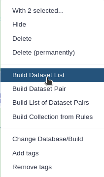
   • Click For all selected.. and choose Build dataset list

     

   • Enter a name for your collection
   • Click Create List to build your collection
   • Click on the checkmark icon at the top of your history again

4. Import the following 2 files from Zenodo or from a shared data library (ask your instructor). Beware: these files must not be in a collection.

   https://zenodo.org/record/3631074/files/sampleMetadata.tsv
   https://zenodo.org/record/3631074/files/W4M0004_database_small.msp
   

   Tip: Importing via links

   • Copy the link location

   • Open the Galaxy Upload Manager (galaxy-upload on the top-right of the tool panel)

   • Select Paste/Fetch Data

   • Paste the link into the text field

   • Press Start

   • Close the window

   Tip: Importing data from a data library

   As an alternative to uploading the data from a URL or your computer, the files may also have been made available from a shared data library:

   • Go into Shared data (top panel) then Data libraries
   • Navigate to the correct folder as indicated by your instructor
   • Select the desired files
   • Click on the To History button near the top and select as Datasets from the dropdown menu
   • In the pop-up window, select the history you want to import the files to (or create a new one)
   • Click on Import

2 - First steps using XCMS

Hands-on: First steps using a standard XCMS workflow

1. MSnbase readMSData Tool: toolshed.g2.bx.psu.edu/repos/lecorguille/msnbase_readmsdata/msnbase_readmsdata/2.16.1+galaxy0 with the following parameters:
   • param-collection “File(s) from your history containing your chromatograms”: mzData (Input dataset collection)
2. xcms findChromPeaks (xcmsSet) Tool: toolshed.g2.bx.psu.edu/repos/lecorguille/xcms_xcmsset/abims_xcms_xcmsSet/3.12.0+galaxy0 with the following parameters:
   • param-file “RData file”: mzData.raw.RData (output of the MSnbase readMSData tool job)
   • “Extraction method for peaks detection”: MatchedFilter - peak detection in chromatographic space
     • “Full width at half maximum of matched filtration gaussian model peak”: 5
     • “Step size to use for profile generation”: 0.5
     • In “Advanced Options”:
       • “Maximum number of peaks that are expected/will be identified per slice”: 500
       • “Signal to Noise ratio cutoff”: 2
       • “Minimum difference in m/z for peaks with overlapping Retention Times”: 0.5

   Comment

   With GC-MS data in profile mode, we need to use the MatchedFilter algorithm instead of the Centwave one used in the LC-MS tutorial.

3. xcms findChromPeaks Merger Tool: toolshed.g2.bx.psu.edu/repos/lecorguille/xcms_merge/xcms_merge/3.12.0+galaxy0 with the following parameters:
   • param-file “RData file”: mzData.raw.xset.RData (output of the xcms findChromPeaks (xcmsSet) tool job)
   • param-file “Sample metadata file “: sampleMetadata.tsv (One of the uploaded files from Zenodo)

   Comment

   To merge your data, you need to input a sampleMetadata file containing filenames and their metadata informations like their class for example. If you don’t add a sampleMetadata file, the xcms findChromPeaks Merger tool tool will group all your files together. You can also create your sampleMetadata file with W4M Galaxy tool xcms get a sampleMetadata file tool with the following parameters: “RData file” outputed from MSnbase readMSData tool. Here is an example of the minimum expectations about a sampleMetadata file (important: don’t write the format of the file, just their names):

   sample_name	class
   file1	man
   file2	woman
   file3	man

The output from xcms findChromPeaks Merger tool is a .RData file that is mandatory to proceed with the end of the extraction process. There are two available options:

• carrying on using the standard XCMS workflow similarly to the one used in the LC-MS tutorial
• using the metaMS strategy specifically designed for GC-MS data The two options are illustrated in this tutorial.

Carrying on using the standard XCMS workflow (option 1)

This option follows the standard LC-MS workflow to obtain in the end a dataMatrix file and its corresponding variableMetadata file.

Hands-on: Example of end of extraction when using the standard XCMS workflow

1. xcms groupChromPeaks (group) Tool: toolshed.g2.bx.psu.edu/repos/lecorguille/xcms_group/abims_xcms_group/3.12.0+galaxy0 with the following parameters:
   • param-file “RData file”: xset.merged.RData (output of the xcms findChromPeaks Merger tool job)
   • “Method to use for grouping”: PeakDensity - peak grouping based on time dimension peak densities
     • “Bandwidth”: 10.0
     • “Width of overlapping m/z slices”: 0.05
2. xcms fillChromPeaks (fillPeaks) Tool: toolshed.g2.bx.psu.edu/repos/lecorguille/xcms_fillpeaks/abims_xcms_fillPeaks/3.12.0+galaxy0 with the following parameters:
   • param-file “RData file”: xset.merged.groupChromPeaks.RData (output of the xcms groupChromPeaks (group) tool job)
   • In “Peak List”:
     • “Convert retention time (seconds) into minutes”: Yes
     • “Number of decimal places for retention time values reported in ions’ identifiers.”: 2
     • “Reported intensity values”: maxo

The outputs of this strategy are similar to the ones discribed in the LC-MS tutotial mentioned previously.

Comment: Important : Be careful of the file format

During each step of pre-processing, your dataset has its format changed and can have also its name changed. To be able to continue to MSMS processing, you need to have a RData object wich is merged and grouped (from xcms findChromPeaks Merger tool and xcms groupChromPeaks (group) tool) at least. It means that you should have a file named xset.merged.groupChromPeaks.RData (and maybe with some step more in it).

Stopover : Verify your data after the XCMS pre-processing

When you have processed all or only needed steps described before, you can continue with the MS/MS processing part with msPurity package. Don’t forget to always check your files format! For the next step you need to have this file xset.merged.groupChromPeaks.*.RData where * is the name of optionnal steps you could do during the pre-processing. For our example, your file should be named xset.merged.groupchromPeaks.RData.

Comment

The pre-processing part of this analysis can be quite time-consuming, and already corresponds to quite a few number of steps, depending of your analysis. We highly recommend, at this step of the MS/MS workflow, to split your analysis by beginning a new Galaxy history with only the files you need (final xset Rdata file and your data collection of mzML). This will help you in limiting selecting the wrong dataset in further analysis, and bring a little tidiness for future review of your MS/MS analysis process. You should also be able to make a better peakpicking in the future in the same history and it will not be polluated by MS/MS part of your process.

Tip: Copy dataset to a new history

1. Click on the galaxy-gear icon (History options) on the top of the history panel
2. Click on Copy Dataset
3. Select the desired files
4. Give a relevant name to the “New history”
5. Click on the new history name in the green box that have just appear to switch to this history

To begin a new history with the files from your current history, you can use the functionality ‘copy dataset’ and copy it into a new history (the option is hidden behind the notched wheel at the top right of the history).

You may have notice that the XCMS tools generate output names that contain the different XCMS steps you used, allowing easy traceability while browsing your history. Hence, we highly recommend you to rename it with something short, e.g. “xset”, “XCMSSetObject”, or anything not too long that you may find convenient.

Tip: Renaming a dataset

• Click on the galaxy-pencil pencil icon for the dataset to edit its attributes
• In the central panel, change the Name field
• Click the Save button

Before the next step with msPurity package on MS/MS datas, here are some questions to be able to verify if your file is ready and if you have the same results as us. Please check these questions :

Question: before MS/MS steps

1 - What are the steps of XCMS you made before your final file ?

Solution

Here are the different steps made for our example :

• (Not with XCMS) import your datas into Galaxy instance
• MSNbase readMSData tool to read our MS datas
• XCMS peakpicking with xcms findChromPeaks (xcmsSet) tool tool
• (Not with XCMS but necessary) merge my datas into one file with xcms findChromPeaks Merger tool tool
• XCMS grouping with xcms groupChromPeaks (group) tool tool
• (Not done) XCMS retention time correction, then grouping again with xcms adjustRtime (retcor) tool tool
• XCMS integration of missing peaks with xcms fillChromPeaks (fillPeaks) tool tool

2 - Concerning what we said before and the previous answer, what is the complete name of your final RData file ?

Solution

During each step of XCMS pre-processing, the name of the file which is processing is completed by the name of the step you were doing. So, finally your file should be name xset.merged.groupChromPeaks.fillChromPeaks.RData. That because (as seen in previous answer) you ran a grouping and the integration after merged datas.

3 - What is the size (in MB) of your final RData file ?

Solution

To be able to see the size of a file in your history, you just have to select it. It will deploy informations about it and you can see the size of yours. For our example, the size of the final file is 1.4 MB.

Processing with metaMS part (option 2)

metaMS is a R package for MS-based metabolomics data. It can do basic peak picking and grouping using functions from XCMS and CAMERA packages. The main output of metaMS is a table of feature intensities in all samples which can be analyzed with multivariate methods immediately. The package also offers the possibility to create in-house databases of mass spectra (including retention information) of pure chemical compounds. These databases can then be used for annotation purposes. The most important functions of this package are runGC and runLC (and each one to create databases createSTDdbGC and createSTDdbLC).

During this tutorial we are interested in GC-MS analysis, so we will use the runGC function of metaMS and described it in details to be able to understand this function. The standard workflow of metaMS for GC-MS data is the following :

The runGC function is implemented in metaMS.runGC tool tool in W4M Galaxy. It takes a vector of file names, corresponding to the samples, and a settings list as mandatory arguments. In addition, some extra arguments can be provided. In particular, a database of standards, as discussed later in the tutorial, can be provided for annotation purposes. This tool regroups all these steps that are described in the following parts to be able to understand all its functionalities and particularities. We will run the tool after we understand each of its steps because it is important to know what are the best parameters for our data and why each parameter is done.

Peak picking

The peak picking is performed by the usual XCMS functions. A function has been written in metaMS to allow the individual parameters to be passed to the function as a settings list. The result is that the whole of the XCMS functionality is available, simply by changing the values of some settings, or by adding fields.

Whereas the package is not up-to-date since the new version of XCMS (3.x). This new version brought a lot of new objects and transformed the peak picking process. To have the last version of this process, metaMS authorized to start its function directly with the file containing all peak picking results.

Due to this update, we have already processed the peak picking during the first part of this tutorial. So we can continue it with the file outputted from the peak picking part. This also allow us to make a good peak picking without the following step include in metaMS functions. So it takes less time of processing and we can verify our peaks with this cut between peak picking and the following steps of GC-MS analysis.

Definition of pseudo-spectra

Rather than a feature-based analysis with individual peaks, as is the case with XCMS, metaMS performs a pseudospectrum-based analysis. So, the basic entity is a set of m/z values showing a chromatographic peak at the same retention time.

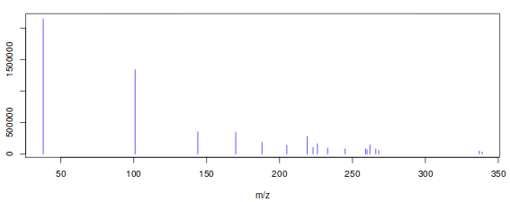
This choice is motivated by several considerations. First of all, in GC the amount of overlap is much less than in LC : peaks are much narrower. This means that even a one- or two-second difference in retention time can be enough to separate the corresponding mass spectra. Secondly, fragmentation patterns for many compounds are available in extensive libraries like the NIST library. In addition, the spectra are somewhat easier to interpret since adducts, such as found in LC, are not present. The main advantage of pseudo-spectra, however, is that their use allows the results to be interpreted directly as relative concentrations of chemical compounds : a fingerprint in terms of chemical composition is obtained, rather than a fingerprint in terms of hard-to-interpret features. The pseudo-spectra are obtained by simply clustering on retention time, using the runCAMERA function, which for GC data calls groupFWHM. All the usual parameters for the groupFWHM function are included in W4M Galaxy metaMS.runGC tool tool. The most important parameter is perfwhm, which determines the maximal retention time difference of features in one pseudospectrum.

The final step is to convert the CAMERA objects into easily handled lists, which are basically the R equivalent of the often-used msp format from the AMDIS software (Stein 1999). The msp file is a nested list, with one entry for each sample, and each sample represented by a number of fields. The pseudo-spectra are three-column matrices, containing m/z, intensity and retention time information, respectively. They can be draw with the plotPseudoSpectrum function of metaMS package easily (Figure 2).

Annotation

Once we have identified our pseudo-spectra, we can start the annotation process. This is done by comparing every pseudospectrum to a database of spectra. As a similarity measure, we use the weighted dot product as it is fast, simple, and gives good results (Stein and Scott 1994). The first step in the comparison is based on retention, since a comparison of either retention time or retention index is much faster than a spectral comparison. The corresponding function is matchSamples2DB. Since the weighted dot product uses scaled mass spectra, the scaling of the database is done once, and then used in all comparisons.

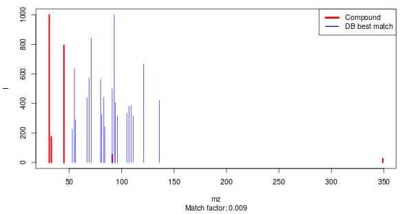
This matchSamples2DB function returns a table where all patterns that have a match with a DB entry are shown in the first column, and the DB entry itself in the second column. If for a particular experimental pattern more than one match is found, the alternatives (with a lower match factor) are shown in the last column. To see the match for a particular pattern, one can use the function matchExpSpec, returning matchfactors (numbers between 0 and 1, where the latter means a perfect match) for all entries in the database (if the plotIt argument is TRUE, the best match is shown – see Figure 2). Samples may contain compounds that are not of any interest, such as plasticizers, internal standards, column material etc…. These can be filtered out before doing an annotation : metaMS allows certain categories of database entries (defined in slot matchIrrelevants of the settings object) to be removed before further annotation. If the spectra of these compounds are very specific (and they often are), the retention criterion may be bypassed by setting the maximal retention time difference to very high values, which leads to the removal of such spectra wherever they occur in the chromatogram.

Unknowns research

The most important aspect of untargeted metabolomics is the definition of unknowns, patterns that occur repeatedly in several samples, but for which no annotation has been found. In metaMS these unknowns are found by comparing all patterns within a certain retention time (or retention index) difference on their spectral characteristics. The same match function is used, but the threshold may be different from the threshold used to match with the database of standards. Likewise, the maximum retention time(index)difference may be different, too.

In defining unknowns we have so far used settings that are more strict than when compared to a database : since all samples are typically measured in one single run, expected retention time differences are rather small. In addition, one would expect reproducible spectra for a single compound. A true unknown, or at least an interesting one, is also present in a significant fraction of the samples. All these parameters are gathered in thebetweenSampleselement of the settingsobject .Since the matching is done using scaled patterns, we need to create a scaled version of the experimental pseudo-spectra first.

For large numbers of samples, this process can take quite some time (it scales quadratically), especiallyif the allowed difference in retention time is large. The result now is a list of two elements : the first is the annotation table that we also saw after the comparison with the database, and the second is a list of pseudo-spectra corresponding to unknowns. In the annotation table, negative indices correspond to the pseudo-spectra in this list.

Outputs and results

At this stage, all elements are complete : we have the list of pseudo-spectra with an annotation, either as a chemical standard from the database, or an unknown occurring in a sizeable fraction of the injections. The only things left to do is to calculate relative intensities for the pseudo-spectra, and to put the results in an easy-to-use table. This table consists of two parts. The first part is the information on the “features”, which here are the pseudo-spectra. The second part of the table contains the intensities of these features in the individual injections.

The first five lines are the standards, and the next ones are the unknowns that are identified by the pipeline. In the manual interpretation of this kind of data, the intensities of one or two “highly specific” features are often used to achieve relative quantitation. In an automatic pipeline, this is a risky strategy: not only can the intensity of a peak vary quite dramatically (relative standard deviations of up to 30% are assumed acceptable in GC-MS, e.g. when SPME is applied), but these errors are all the more pronounced in high-intensity peaks (hence the common use of a relative standard deviation).

In addition, one is ignoring the information in the other peaks of the pseudospectrum. In metaMS, pseudospectrum intensity is expressed as a multiple of the corresponding reference pattern (either a database pattern or an unknown), where the intensity ratio is determined using robust regression to avoid one deviating feature to influence the results too much (Wehrens et al. 2014). First, we define an object containing all relevant pseudo-spectra, and next the intensities are generated.

In both cases, the result is a list containing a set of patterns corresponding with the compounds that have been found, either annotated or unknown, the relative intensities of these patterns in the individual annotations, and possibly the xcmsSetobject for further inspection. In practice, the runGC function is all that users need to use.

That file can be used for database search online (as Golm (J. et al. 2005) and MassBank (Hisayuki et al. 2010)) or locally (NIST MSSEARCH) for NIST search a tutorial is available here.

Hands-on: metaMS.runGC

We now know each step of this runGC function. So, please open the metaMS.runGC tool too to run it. You should enter the following parameters for our tutorial :

• Rdata from xcms and merged : here you have to select your file from XCMS where you made the peak picking, grouping and all the pre-processing. It should be named xset.merged.groupdChromPeaks.RData.
• Settings : you can keep it at user_default but to see all possible parameters please set it at use_defnied.
  • RT range option : it ables to select a region of retention time. If you select to show it, you have to enter the window in minutes, separate by a coma (for example 5,20 to have results between 5 minutes and 20 minutes). For our tutorial, we keep it to hide.
  • RT_Diff : it is the allowed retention time difference in minutes between the same compound/unknown in different sample. For our tutorial, keep it at 0.05 to have low differences between unknowns’ retention times.
  • Min_Features : this parameter is used during the comparison with database or unknowns. It corresponds to the minimal number of features required to have a valid pseudospectrum. For our tutorial, please keep it to 5 to have really good compounds.
  • similarity_threshold : this parameter is also used for comparison. It is the minimum similarity allowed between peaks mass spectra to be considers as equal. For our tutorial, please keep it to 0.7.
  • min.class.fract : it corresponds to the minimal fraction of samples in which a pseudospectrum is present before it is regarded as an unknown. For the tutorial, please keep it to 0.5.
  • min.class.size : it corresponds to the minimum number of samples in which a pseudospectrum should be present before it is regarded as an unknown. For our tutorial, please set it to 2 because we have classes with only 2 samples.
• Use Personnal DataBase option : you can compare your datas to a personnal database. If you want to do it start to choose show in this parameter. Then you will be able to select your file. If not, keep it to hide and you will only have unknowns as results.
  • DB file : this parameter will appear if you choose to show it. You just have to select your database in your file to add this here. Be careful, this database has to respect some rules (please look at ?????????????????? part).
• Use RI option : choose if you want to use the RI for standards.
  • RI file : enter here your RI file which have to contains two columns : retention time and retention indices.
• Use RI as filter : just to know if you want to use RI parameter as a filter.
  • RIshift : if you want to use RI as filter, please precise here the RI shift. For our tutorial keep the previous parameter to FALSE.

Take a look at your results after metaMS processing

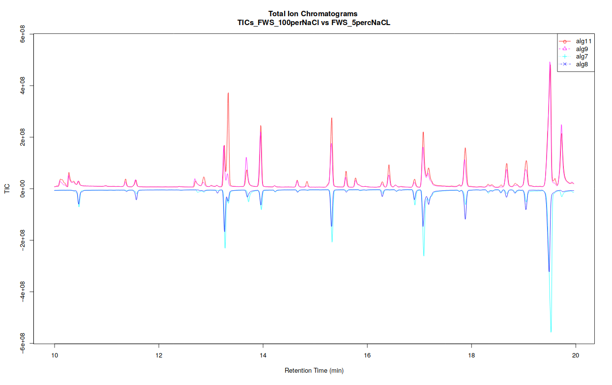
We choose to separate our first W4M Galaxy tool into 2 parts: the processing of GC-MS data (metaMS.runGC tool) and the plotting results of these data (metaMS.plot tool). So we now have the first part describes just before and the second part we will describe just after. This part allows users to see the TIC (Total Ion Chromatogram), BPC (Base Peak Chromatogram), and also all EICs (Extracted Ion Chromatogram) you want, from our previous result outputted from metaMS.runGC tool tool.

If you separated your samples into different classes, this tool can constructs TICs and BPCs one class against one class, in a pdf file (Figure 5) :

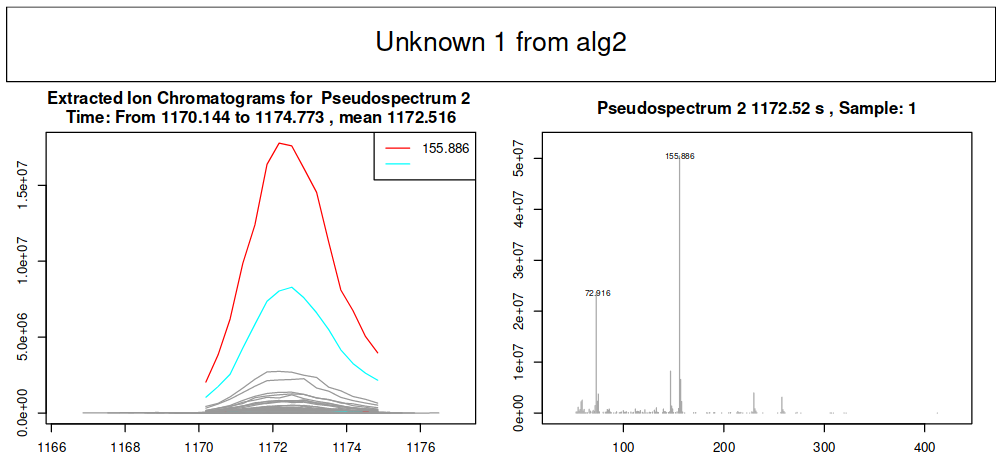
Concerning EICs, it is possible to choose for which compound you want to draw an EIC when you run the W4M Galaxy tool. According to your choice, you will obtain EICs for one compound in each sample you enter in the previous metaMS part.

Hands-on: metaMS.plot

This tool is very easy to run. It is an obligation to process metaMS.runGC tool before this one. After that, you just have to choose if you want or not to draw your TIC, BPC or EIC :

• Rdata from new_metaMS_runGC : the file you obtained with the metaMS.runGC tool tool. It should be named runGC.RData.
• Do you want to process for TIC(s) ? : if you select “yes” you will obtain the pdf file containing each TIC from each class against each others.
• Do you want to process for BPC(s) ? : if you select “yes” you will obtain the pdf file containing each BPC from each class against each others.
• Do you want to process for EIC(s) ? : if you select “yes” you will have to choose which compound(s) and unknown(s) you want to obtain its EIC.
  • EIC_Unknown : here please choose which compound(s) or unknown(s) you want to obtain according to the peaktable.tsv file. For out tutorial it can be interesting to have a look at all the EICs. So put the value to 0.

Conclusion

Key points

• Have a good file containing all your peaks during the first stopover

• Find all your unknowns in your datas

• Find your stanards if you have some

Frequently Asked Questions

Have questions about this tutorial? Check out the tutorial FAQ page or the FAQ page for the Metabolomics topic to see if your question is listed there. If not, please ask your question on the GTN Gitter Channel or the Galaxy Help Forum

References

1. Stein, S. E., and D. R. Scott, 1994 Optimization and testing of mass spectral library search algorithms for compound identification. Journal of the American Society for Mass Spectrometry 5: 859–866. 10.1016/1044-0305(94)87009-8
2. Stein, S. E., 1999 An integrated method for spectrum extraction and compound identification from gas chromatography/mass spectrometry data. Journal of the American Society for Mass Spectrometry 10: 770–781. 10.1016/S1044-0305(99)00047-1
3. J., K., S. N., K. S., B. C., U. B. et al., 2005 GMD@CSB.DB: the Golm Metabolome Database. Bioinformatics 21: 1635–1638. 10.1093/bioinformatics/bti236 http://gmd.mpimp-golm.mpg.de/
4. Smith, C. A., E. J. Want, G. O’Maille, R. Abagyan, and G. Siuzdak, 2006 XCMS:  Processing Mass Spectrometry Data for Metabolite Profiling Using Nonlinear Peak Alignment, Matching, and Identification. Analytical Chemistry 78: 779–787. 10.1021/ac051437y
5. Hisayuki, H., A. Masanori, K. Shigehiko, N. Yoshito, I. Tasuku et al., 2010 MassBank: a public repository for sharing mass spectral data for life sciences. Journal of Mass Spectrometry 45: 703–714. 10.1002/jms.1777 https://massbank.eu/MassBank/Search
6. Dittami, S. M., A. Gravot, S. Goulitquer, S. Rousvoal, A. F. Peters et al., 2012 Towards deciphering dynamic changes and evolutionarymechanisms involved in the adaptation to low salinities inEctocarpus(brown algae). The Plant Journal 71: 366–377. 10.1111/j.1365-313X.2012.04982.x
7. Wehrens, R., G. Weingart, and F. Mattivi, 2014 metaMS: An open-source pipeline for GC-MS-based untargeted metabolomics. Journal of Chromatography B 966: 109–116. 10.1016/j.jchromb.2014.02.051
8. Carsten Kuhl, R. T., 2017 CAMERA. 10.18129/b9.bioc.camera https://bioconductor.org/packages/CAMERA

Feedback

Did you use this material as an instructor? Feel free to give us feedback on how it went.
Did you use this material as a learner or student? Click the form below to leave feedback.

Citing this Tutorial

1. Julien Saint-Vanne, 2022 Mass spectrometry : GC-MS analysis with metaMS package (Galaxy Training Materials). https://training.galaxyproject.org/training-material/topics/metabolomics/tutorials/gcms/tutorial.html Online; accessed TODAY
2. Batut et al., 2018 Community-Driven Data Analysis Training for Biology Cell Systems 10.1016/j.cels.2018.05.012

BibTeX

@misc{metabolomics-gcms,
author = "Julien Saint-Vanne",
title = "Mass spectrometry : GC-MS analysis with metaMS package (Galaxy Training Materials)",
year = "2022",
month = "10",
day = "18"
url = "\url{https://training.galaxyproject.org/training-material/topics/metabolomics/tutorials/gcms/tutorial.html}",
note = "[Online; accessed TODAY]"
}
@article{Batut_2018,
    doi = {10.1016/j.cels.2018.05.012},
    url = {https://doi.org/10.1016%2Fj.cels.2018.05.012},
    year = 2018,
    month = {jun},
    publisher = {Elsevier {BV}},
    volume = {6},
    number = {6},
    pages = {752--758.e1},
    author = {B{\'{e}}r{\'{e}}nice Batut and Saskia Hiltemann and Andrea Bagnacani and Dannon Baker and Vivek Bhardwaj and Clemens Blank and Anthony Bretaudeau and Loraine Brillet-Gu{\'{e}}guen and Martin {\v{C}}ech and John Chilton and Dave Clements and Olivia Doppelt-Azeroual and Anika Erxleben and Mallory Ann Freeberg and Simon Gladman and Youri Hoogstrate and Hans-Rudolf Hotz and Torsten Houwaart and Pratik Jagtap and Delphine Larivi{\`{e}}re and Gildas Le Corguill{\'{e}} and Thomas Manke and Fabien Mareuil and Fidel Ram{\'{\i}}rez and Devon Ryan and Florian Christoph Sigloch and Nicola Soranzo and Joachim Wolff and Pavankumar Videm and Markus Wolfien and Aisanjiang Wubuli and Dilmurat Yusuf and James Taylor and Rolf Backofen and Anton Nekrutenko and Björn Grüning},
    title = {Community-Driven Data Analysis Training for Biology},
    journal = {Cell Systems}
}
                   

Congratulations on successfully completing this tutorial!