Agenda

In this tutorial we will do:

1. quality control
2. alignment
3. methylation extraction
4. visualization of methylation levels
5. differentially methylated regions analysis

We will use a small subset of the original data. If we would do the computation on the orginal data the computation time for a tutorial is too long. To show you all necessary steps for Methyl-Seq we decided to use a subset of the data set. In a second step we use precomputed data from the study to show you different levels of methylation. We will consider samples from normal breast cells (NB), fibroadenoma (noncancerous breast tumor, BT089), two invasive ductal carcinomas (BT126, BT198) and a breast adenocarcinoma cell line (MCF7).

This tutorial is based off of Lin et al. 2015. The data we use in this tutorial is available at Zenodo.

Load data and quality control

Hands-on: Get the data and look at the quality

We load now the example dataset which will be used for the tutorial.

1. Load the two example datasets from our data library: subset_1.fastq.gz and subset_2.fastq.gz.

   Tip: Get data from the library

   • Click on Shared Data –> Data Libraries and here MethylSeq_2017
   • Select the uploaded datasets subset_1.fastq.gz and subset_2.fastq.gz as the fastq files

2. Quality control

   Tip: Search for tools

   • FastQC tool with the following parameters:
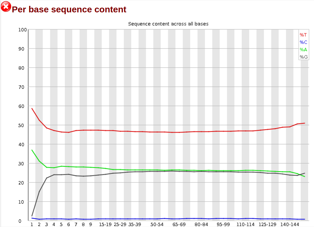
   • Select the uploaded datasets subset_1.fastq.gz and subset_2.fastq.gz as the fastq files

3. Go to the web page result page and have a closer look at ‘Per base sequence content’

   

   Question

   1. Note the GC distribution and percentage of “T” and “C”. Why is this so weird?
   2. Is everything as expected?

   Solution

   1. The attentive audience of the theory part knows: Every C-meth stays a C and every normal C becomes a T during the bisulfite conversion.
   2. Yes it is. Always be careful and have the specific characteristics of your data in mind during the interpretation of FastQC results.

Alignment

Hands-on: Mapping with bwameth

We will map now the imported dataset against a reference genome.

1. bwameth tool with the following parameters:
   • Select for the option Select a genome reference from your history or a built-in index? Use a built-in index and here the human hg38 genome.
   • Choose for the option Is this library mate-paired? Paired-end and use the two imported datasets as an input. Compute now the alignment. Please notice that depending on your system this computation can take some time. If you want to skip this, we provide for you a precomputed alignment. Import aligned_subset.bam to your history.

   Question

   Why we need other alignment tools for bisulfite sequencing data?

   Solution

   You may have noticed that all the C’s are C-meth’s and a T can be a T or a C. A mapper for methylation data needs to find out what is what.

Methylation bias and metric extraction

Hands-on: Methylation bias

In this step we will have a look at the distribution of the methylation and will look at a possible bias.

1. MethylDackel tool with the following parameters:
   • Choose at the first option Load reference genome from Local cache and for Using reference genome the value hg38.
   • Select for the option sorted_alignments.bam the computed bam file of step 4 of the bwameth alignment.
   • Use for What do you want to do? the value Determine the position-dependent methylation bias in the dataset, producing diagnostic SVG images.
   • Set the parameters By default, if only one read in a pair aligns (a singleton) then it's ignored. and By default, paired-end alignments with the properly-paired bit unset in the FLAG field are ignored. Note that the definition of concordant and discordant is based on your aligner settings. to Yes.

   

   Question

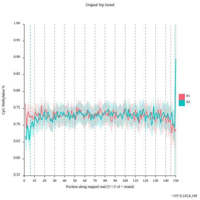
   1. Consider the original top strand output. Is there a methylation bias?
   2. If we would trim, what would be the start and the end positions?

   Solution

   1. The distribution of the methylation is more or less equal. Only at the start and the end we could trim a bit but a +- 5% variation is acceptable.
   2. To trim the reads we would include for the first strand only the positions 0 to 145, for the second 6 to 149.

Hands-on: Methylation extraction with MethylDackel

We will extract the methylation on the resulting BAM file of the alignment step. We need this to create a methylation level plot in the next step.

1. MethylDackel tool with the following parameters:
   • Choose at the first option Load reference genome from the value: Local cache and for Using reference genome the value: hg38.
   • Select for the option sorted_alignments.bam the computed bam file of step 4 of the bwameth alignment.
   • Use for What do you want to do? the value Extract methylation metrics from an alignment file in BAM/CRAN format.
   • Choose Yes for the option Merge per-Cytosine metrics from CpG and CHG contexts into per-CPG or per-CHG metrics.
   • Set the parameter Extract fractional methylation (only) at each position. This is mutually exclusive with --counts, --logit, and --methylKit to Yes.
   • All other options use the default value.

Visualization

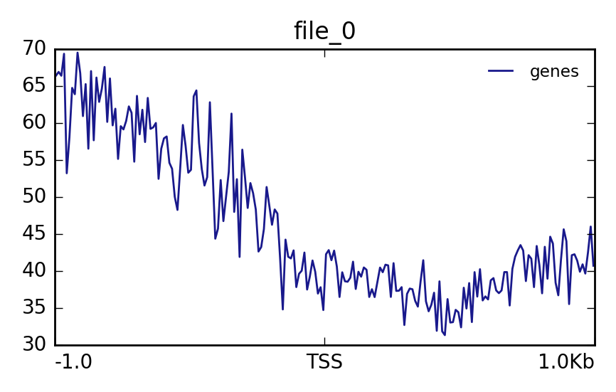
Hands-on

In this step we want to visualize the methylation level around all TSS of our data. When located at gene promoters, DNA methylation is usually a repressive mark.

1. Wig/BedGraph-to-bigWig tool with the following parameters:

   • Use the result of MethylDackel to transform it to a bigWig file.

     Tip: Database edit

     It can happen that you can not select the correct input file. In this case you have to add meta information about the used genome to the file.

     • Click on the pencil of the correct history item.
     • Change Database/Build: to the genome you used.
     • In our case the correct genome is Human Dec. 2013 (GRCh38/hg38) (hg38).

2. computeMatrix tool with the following parameters:
   • Use the file CpGIslands.bedas Regions to plot and the in the previous step created bigwig file as the score file.
   • Use for the option computeMatrix has two main output options the value reference-point.
3. plotProfile tool with the following parameters:
   • Choose for Matrix file from the computeMatrix tool the computed matrix from the tool computeMatrix.

The output should look like this:

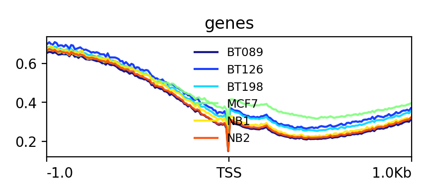
Lets see how the methylation looks for a few provided files:

1. Galaxy tool: Import the files NB1_CpG.meth.bedGraph from the data library
2. Wig/BedGraph-to-bigWig tool with the following parameters:
   • Use the imported file to transform it to a bigWig file.

   Question

   The execution fails. Do you have an idea why?

   Solution

   A conversion to bigWig would fail right now, probably with some error message like hashMustFindVal: '1' not found. The reason is the source of the reference genome which was used. There is ensembl and UCSC as sources which differ in naming the chromosomes. Ensembl is using just numbers e.g. 1 for chromosome one. UCSC is using chr1 for the same. Be careful with this especially if you have data from different sources. We need to convert this.

   Comment: UCSC - Ensembl convert

   • Download the Replace information file for hg38 chromosome: Download and import it to Galaxy.
   • Replace column tool:
     • Choose for File in which you want to replace some values the previous used NB1_CpG.meth.bedGraph file and for Replace information file conversion file. For Which column should be replaced? choose Column: 1, for Skip this many starting lines a 1 and for Delimited by Tab.

3. To save compute time we prepared the converted files for you. Import the files: NB1_CpG.meth_ucsc.bedGraph, NB2_CpG.meth_ucsc.bedGraph, BT089_CpG.meth_ucsc.bedGraph, BT126_CpG.meth_ucsc.bedGraph, BT198_CpG.meth_ucsc.bedGraph and MCF7_CpG.meth_ucsc.bedgraph.
4. Compute the matrix and plot the profile as described above.

More information about deepTools can be found here: https://deeptools.readthedocs.io

Metilene

Hands-on: Metilene

With metilene it is possible to detect differentially methylated regions (DMRs) which is a necessary prerequisite for characterizing different epigenetic states.

1. Galaxy tool: Import from the data library the files NB1_CpG.meth.bedGraph, NB2_CpG.meth.bedGraph and BT198_CpG.meth.bedGraph.
2. Metilene tool:
   • Choose for the first option Input group 1 the imported files starting with NB and for Input group 2 the imported files BT198_CpG.meth.bedGraph.
   • Select for the option BED file containing regions of interest the imported BED file CpGIslands.bed.

3. More information about metilene can be found here: https://www.bioinf.uni-leipzig.de/Software/metilene

   Question

   Have a look at the produced pdf document. What is the data showing?

   Solution

   It shows the distribution of DMR differences, DMR length in nucleotides and number CpGs, DMR differences vs. q-values, mean methylation group 1 vs. mean methylation group 2 and DMR length in nucleotides vs. length in CpGs

Key points

• The output of a methylation NGS is having a different distribution of the four bases. This is caused by the bisulfite treatment of the DNA.

• If there is a different level of methylation in the loci of a gene this can be a hint that something is wrong.

• To get useful results you need – data, data and data!

Frequently Asked Questions

Have questions about this tutorial? Check out the tutorial FAQ page or the FAQ page for the Epigenetics topic to see if your question is listed there. If not, please ask your question on the GTN Gitter Channel or the Galaxy Help Forum

References

1. Lin, I.-H., D.-T. Chen, Y.-F. Chang, Y.-L. Lee, C.-H. Su et al., 2015 Hierarchical Clustering of Breast Cancer Methylomes Revealed Differentially Methylated and Expressed Breast Cancer Genes (O. El-Maarri, Ed.). PLOS ONE 10: e0118453. 10.1371/journal.pone.0118453

Feedback

Did you use this material as an instructor? Feel free to give us feedback on how it went.
Did you use this material as a learner or student? Click the form below to leave feedback.

Citing this Tutorial

1. Joachim Wolff, Devon Ryan, 2022 DNA Methylation data analysis (Galaxy Training Materials). https://training.galaxyproject.org/training-material/topics/epigenetics/tutorials/methylation-seq/tutorial.html Online; accessed TODAY
2. Batut et al., 2018 Community-Driven Data Analysis Training for Biology Cell Systems 10.1016/j.cels.2018.05.012

BibTeX

@misc{epigenetics-methylation-seq,
author = "Joachim Wolff and Devon Ryan",
title = "DNA Methylation data analysis (Galaxy Training Materials)",
year = "2022",
month = "09",
day = "28"
url = "\url{https://training.galaxyproject.org/training-material/topics/epigenetics/tutorials/methylation-seq/tutorial.html}",
note = "[Online; accessed TODAY]"
}
@article{Batut_2018,
    doi = {10.1016/j.cels.2018.05.012},
    url = {https://doi.org/10.1016%2Fj.cels.2018.05.012},
    year = 2018,
    month = {jun},
    publisher = {Elsevier {BV}},
    volume = {6},
    number = {6},
    pages = {752--758.e1},
    author = {B{\'{e}}r{\'{e}}nice Batut and Saskia Hiltemann and Andrea Bagnacani and Dannon Baker and Vivek Bhardwaj and Clemens Blank and Anthony Bretaudeau and Loraine Brillet-Gu{\'{e}}guen and Martin {\v{C}}ech and John Chilton and Dave Clements and Olivia Doppelt-Azeroual and Anika Erxleben and Mallory Ann Freeberg and Simon Gladman and Youri Hoogstrate and Hans-Rudolf Hotz and Torsten Houwaart and Pratik Jagtap and Delphine Larivi{\`{e}}re and Gildas Le Corguill{\'{e}} and Thomas Manke and Fabien Mareuil and Fidel Ram{\'{\i}}rez and Devon Ryan and Florian Christoph Sigloch and Nicola Soranzo and Joachim Wolff and Pavankumar Videm and Markus Wolfien and Aisanjiang Wubuli and Dilmurat Yusuf and James Taylor and Rolf Backofen and Anton Nekrutenko and Björn Grüning},
    title = {Community-Driven Data Analysis Training for Biology},
    journal = {Cell Systems}
}
                   

Congratulations on successfully completing this tutorial!